How Robust Is PID Control? Testing Inertia, Sensor Noise, and Delay in MuJoCo
The same PID gains, the same pendulum — now with uncertain inertia, noisy sensors, and late observations
Day 2 ended with a controller that worked. A reusable scalar PID held a MuJoCo pendulum at +30°: it settled 3.630 seconds after the step, with a final-window mean absolute error of 0.313°. P and PI oscillated and never settled; PD kept a gravity offset. Only PID settled, and the numbers said so.
That was a clean simulation. The controller saw the true angle, instantly, every 10 milliseconds. Nothing in Day 2 tested what happens when that stops being true.
Day 3 asks the obvious next question: our PID controller worked in a clean simulation — what happens when the model is uncertain, sensor measurements are noisy, or observations arrive late? Same gains, same pendulum, same step. Three sources of uncertainty, one at a time, then all three at once.
The short answer: the fixed gains tolerated the inertia and delay changes without a single failed or unsettled run. Sensor noise was the real story — not because the pendulum stopped tracking, but because the controller started thrashing. And the combined case produced the one result none of the single-factor cases did: overshoot.
There is still no walking robot, no learned policy, and no hardware. What exists is a reproducible simulation, measured numbers, and an observation pipeline you can reuse.
1. What Day 2 Actually Proved
Before testing robustness, it helps to say exactly what the baseline is — because every Day 3 number is a comparison against it.
Day 2's experiment was a step response. The pendulum starts at 0°, the target steps to +30° at 0.5 seconds, and the run lasts 10 seconds. The PID gains are Kp=6, Ki=3, Kd=1, with torque limited to ±3 N·m. The controller decides every 10 ms; the physics runs at 2 ms with RK4 integration.
The baseline result, reproduced exactly in Day 3's zero-noise, zero-delay run:
| Metric | Baseline |
|---|---|
| Final-window MAE (mean absolute error, last 2 s) | 0.313° |
| Post-step RMSE (0.5–10 s) | 4.300° |
| Overshoot above +30° | 0.000° |
| Settling time (within ±2°, after the step) | 3.630 s |
| RMS change between adjacent commands | 0.099 N·m |
| Saturation (commands beyond ±3 N·m) | 0.1% |
"Settling" has a strict meaning here: the angle must stay within ±2° of the target for every subsequent physics sample. A settling time of null would mean the response never stayed inside the band — it is never converted to zero. Final-window MAE covers only the last two seconds (8–10 s); it is a finite-window statistic, not a guaranteed steady-state error.
The gravity holding torque at +30° is 1.22625 N·m — the motor must continuously supply that just to hold still:
Day 2 proved one thing: with perfect information, this gain set works. Day 3 tests whether it keeps working when the information stops being perfect.
2. Three Sources of Uncertainty
A real robot joint never matches its model exactly, never measures perfectly, and never hears about the present instantly. For a humanoid, interchangeable limbs will have different inertia, sensing, and timing — that is the whole point of building the robot modular. So Day 3 tests the three mismatches that matter most for a single hinge:
Inertia. The model's hinge inertia is 0.086392578125 kg·m², compiled from a 1 kg, 0.5 m capsule. A real limb could be heavier, or carry its mass differently. If the controller was tuned for one inertia, what happens at 1.5× or 2×?
Sensor noise. A real angle sensor reports the truth plus noise. The controller in Day 2 differentiated the measurement itself — the derivative term reacts to how fast the measured angle changes. Noise between two consecutive measurements goes straight into that term.
Observation delay. A real measurement takes time to travel from sensor to controller. By the time the controller acts, the angle it sees is already old. Fixed delays of 10, 30, and 50 ms are small in absolute terms — five controller updates at most — but feedback running on stale data is a classic way to lose stability.
Each of these is a different kind of wrongness: the model is wrong, the measurement is wrong, the timing is wrong. Testing them separately matters, because if you change all three at once and something breaks, you cannot say which one broke it.
3. Designing a Controlled Experiment
The design is one factor at a time, plus one combined case. Nine scenarios, same everything else:
SCENARIOS = (
    Scenario("baseline"),
    Scenario("inertia_1_5x", inertia_factor=1.5),
    Scenario("inertia_2x", inertia_factor=2.0),
    Scenario("noise_0_2deg", noise_sd_deg=0.2),
    Scenario("noise_0_4deg", noise_sd_deg=0.4),
    Scenario("delay_10ms", delay_ms=10),
    Scenario("delay_30ms", delay_ms=30),
    Scenario("delay_50ms", delay_ms=50),
    Scenario("combined", inertia_factor=2.0, noise_sd_deg=0.4, delay_ms=50),
)
Every case keeps the Day 2 setup: 1 kg body, −9.81 m/s² gravity, RK4, 0.002 s physics step, 0.01 s controller step, ±3 N·m torque, 0° initial state, +30° step at 0.5 s, 10 s duration, Kp=6, Ki=3, Kd=1. No gains were retuned. That is the design: robustness here means the same controller coping with a different world, not a controller re-tuned for each world.
Stochastic cases (the noise cases and the combined case) run five seeds — 11, 23, 37, 53, 71 — and report the mean and the observed range. Deterministic cases run seed 11 only. Noise is independent zero-mean Gaussian angle noise, drawn once per controller decision; it enters only the controller's observation and never changes MuJoCo's true state. Delays are fixed and must be multiples of the 10 ms update interval.
Here is the full result table. All errors use MuJoCo ground-truth angle, even when the controller saw something else:
| Scenario | Final MAE ° mean [range] | RMSE ° mean | Overshoot ° mean | Settling s mean [range] | RMS torque change N·m | Saturation mean |
|---|---|---|---|---|---|---|
| Baseline | 0.313 [0.313, 0.313] | 4.300 | 0.000 | 3.630 | 0.099 | 0.1% |
| Inertia 1.5× | 0.319 [0.319, 0.319] | 4.468 | 0.000 | 3.674 | 0.098 | 0.2% |
| Inertia 2× | 0.320 [0.320, 0.320] | 4.608 | 0.000 | 3.680 | 0.097 | 0.2% |
| Noise 0.2° | 0.308 [0.282, 0.321] | 4.314 | 0.000 | 3.650 [3.586, 3.726] | 0.888 | 0.14% |
| Noise 0.4° | 0.390 [0.307, 0.485] | 4.396 | 0.027 | 4.152 [3.792, 4.364] | 1.715 | 3.9% |
| Delay 10 ms | 0.315 [0.315, 0.315] | 4.256 | 0.000 | 3.648 | 0.100 | 0.2% |
| Delay 30 ms | 0.318 [0.318, 0.318] | 4.184 | 0.000 | 3.684 | 0.102 | 0.4% |
| Delay 50 ms | 0.321 [0.321, 0.321] | 4.177 | 0.000 | 3.718 | 0.109 | 0.6% |
| Combined | 0.395 [0.298, 0.496] | 4.649 | 1.477 | 4.190 [3.838, 4.494] | 1.680 | 4.1% |
A note on what "robustness" means in this article and what it does not. It means: these nine measured runs, with these gains, on this pendulum. It does not mean a guarantee for other gains, other targets, other seeds, or hardware. Every number below is a measurement from summary.json, not a claim about robots in general.
4. Experiment A — Changing Inertia
The inertia change is deliberately narrow. PendulumModelConfig(inertia_factor=...) increases the two transverse central body inertia components by the same amount, so the compiled effective hinge inertia becomes 0.1295888671875 kg·m² at 1.5× and 0.17278515625 kg·m² at 2×. Body mass, center of mass, gravity, damping, actuator gear, and torque range are all unchanged — and the +30° gravity holding torque stays exactly 1.22625 N·m in all three cases.
That isolation is the point, and also the limit. A real heavier limb would change mass, center of mass, and holding torque together. Here only rotational inertia changes, so the experiment answers one question: how sensitive is this controller to inertia alone? The visible capsule geometry is unchanged even though the inertia tensor now represents a different mass distribution, so this is an idealized sensitivity test, not a redesigned physical rod.
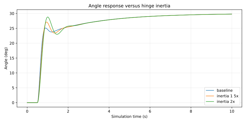
Figure: seed-11 angle traces for baseline, 1.5×, and 2× hinge inertia. The three curves are nearly on top of each other; the difference is in the numbers, not the shape.
The result is almost boring — and that is informative. Doubling inertia moved final-window MAE from 0.313° to 0.320°, and settling from 3.630 s to 3.680 s: 50 milliseconds slower on a 3.6-second settle. Post-step RMSE rose more visibly, from 4.300° to 4.608°, because the heavier pendulum takes a slightly different path to the target even though it ends up in the same place. Overshoot stayed at zero in all three cases, and the command-change RMS actually fell slightly (0.099 → 0.097 N·m), because a heavier pendulum responds more slowly to each command.
Do not read this as "doubling a real robot arm's mass has no effect." The holding torque did not change here; in a real arm it would. What the experiment says is narrower: with the same gains and the same holding torque, this controller's steady accuracy barely notices a 2× inertia error. The transient notices a little more. That is a useful property for interchangeable limbs — but only for the inertia part of the difference.
5. Experiment B — Sensor Noise
This is the experiment that changed how I think about the controller. The mechanism is in one line of the PID code — the derivative term is derivative-on-measurement:
derivative = (
    0.0 if self.previous_measurement is None
    else -(measurement - self.previous_measurement) / dt
)
The D term does not differentiate the error. It differentiates the measurement itself: how fast the angle the controller sees is changing. With clean measurements that is fine. With noisy ones, the difference between two consecutive measurements is mostly noise — and dividing by dt = 0.01 s multiplies it by 100.
You can predict the size of that effect before running anything. If each measurement carries independent Gaussian noise with standard deviation σ, the difference of two consecutive measurements has standard deviation , and dividing by the update interval gives a derivative-noise scale of . For σ = 0.4°:
The measured derivative-input error RMS was 0.974 rad/s — within 1.5% of that prediction. For 0.2° noise the prediction is 0.494 rad/s and the measurement was 0.487 rad/s. The theory is not subtle; it is arithmetic, and the simulation agrees with it.
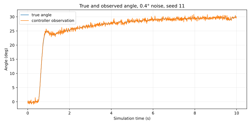
Figure: true angle (blue) against the controller's observation (orange) under 0.4° noise, seed 11. The observation jitters ±0.4° around the truth at every update. The raw sensor error RMS is 0.400°, exactly the injected noise level.
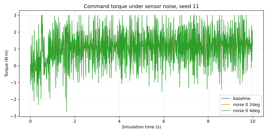
Figure: commanded torque for baseline, 0.2° noise, and 0.4° noise, seed 11. The baseline command is smooth; the 0.4° case chatters across nearly the full ±3 N·m range for the whole run.
The consequences show up in the command, not in the final angle. At 0.4° noise, the five-seed mean final-window MAE was 0.390° — worse than baseline, but the pendulum still settled in every seed (mean 4.152 s, range 3.792–4.364 s). What exploded was the command: RMS change between adjacent commands rose from 0.099 N·m at baseline to 1.715 N·m, a 17× increase, and saturation rose from 0.1% to 3.9% of controller decisions. Total RMS torque rose from 1.124 to 1.504 N·m.
Be precise about what that 1.715 N·m is: it is the RMS of the change between consecutive commands, not total motor torque, not electrical energy, and not measured physical wear. It measures how violently the command signal itself fluctuates. On a real motor that fluctuation would mean heat, vibration, and wear — but this simulation has no motor model, so the number is a warning sign, not a wear measurement.
One result deserves a warning in the opposite direction. At 0.2° noise, the five-seed mean final-window MAE was 0.308° — slightly lower than the no-noise baseline of 0.313°. It would be tempting to say a little noise helps. It does not establish that. Five seeds over a 10-second window is not enough to claim noise improves control, and the same case's command-change RMS (0.888 N·m) was already nine times baseline. The honest reading: at 0.2° the tracking error is roughly unchanged while the command is already much rougher.
6. Experiment C — Fixed Observation Delay
Delay works differently from noise. Noise corrupts the value; delay corrupts the timing. The observation pipeline keeps a causal history of timestamped samples and returns the newest sample at or before decision time minus the requested delay. Before a full history exists, it holds the t=0 sample — so during startup the measurement is younger than the requested delay. For the 50 ms case, the mean measurement age across decisions was 49.85 ms.
def observe(self, decision_time_s: float, true_angle_rad: float) -> Observation:
    if not isfinite(true_angle_rad):
        raise ValueError("true angle must be finite")
    raw = true_angle_rad + (self.rng.gauss(0.0, self.noise_sd_rad)
                            if self.noise_sd_rad else 0.0)
    self.history.append(decision_time_s, raw)
    measurement_time, angle = self.history.at(decision_time_s)
    return Observation(angle, raw, measurement_time, decision_time_s - measurement_time)
The controller sees the delayed value. The metrics always use the true state — otherwise a controller that tracks a stale target would look good by measuring against the same stale target.
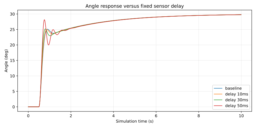
Figure: seed-11 angle traces for baseline and 10, 30, and 50 ms fixed delays. The delayed curves lag the baseline slightly and settle slightly later; the shape is otherwise the same.
The delay results are the most counterintuitive in the study. Settling got slower with delay, as expected: 3.648 s at 10 ms, 3.684 s at 30 ms, 3.718 s at 50 ms, against 3.630 s baseline. But post-step RMSE decreased with delay: 4.300° at baseline, 4.256° at 10 ms, 4.184° at 30 ms, 4.177° at 50 ms. Final-window MAE barely moved (0.315°, 0.318°, 0.321°).
That is a measured tradeoff for this one transient, not evidence that delay improves control. A delayed observation slightly smooths the early response — the controller reacts to where the pendulum was, which in this particular step happens to reduce the overall squared error — while the final approach takes longer. Overshoot stayed at zero and saturation stayed low (0.2–0.6%). The lesson is narrower and more useful: a fixed 50 ms delay did not destabilize this controller, but the metric that improved (RMSE) and the metric that worsened (settling) measure different things, and quoting only one of them would mislead.
7. Combined Disturbances
The combined case is one selected configuration, not a sweep: 2× inertia, 0.4° noise, and 50 ms delay together, five seeds. It is the only case where the three uncertainties interact, and the only case where anything qualitatively new appeared.
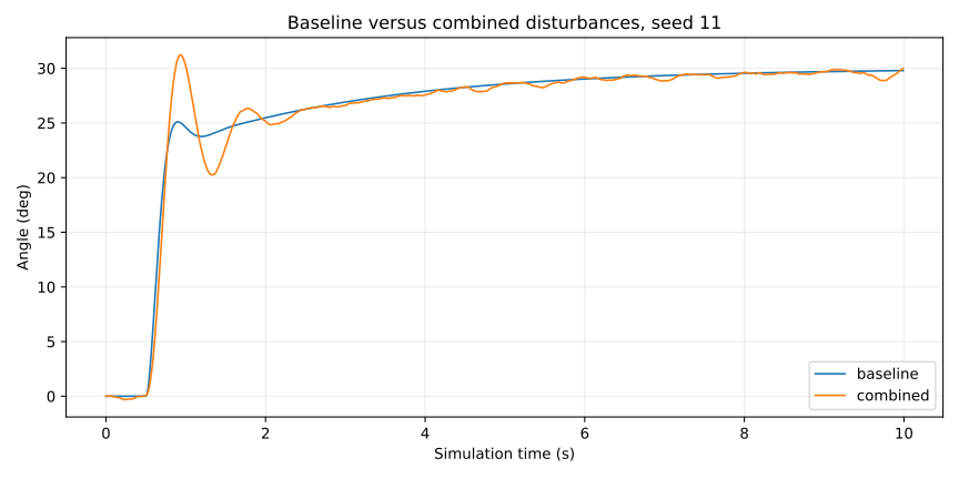
Figure: seed-11 angle traces for baseline and the combined case (2× inertia, 0.4° noise, 50 ms delay). The combined trace overshoots past +30°, dips, and oscillates before settling — behavior none of the single-factor cases showed.
The numbers: five-seed mean final-window MAE 0.395° (range 0.298–0.496°), mean settling 4.190 s (range 3.838–4.494 s), mean overshoot 1.477° (range 1.248–1.910°), command-change RMS 1.680 N·m, saturation 4.1%. Every seed settled within 10 seconds and stayed finite.
The overshoot is the signal. Every single-factor case had zero overshoot — including 0.4° noise alone, which had a mean overshoot of only 0.027°. Put the three factors together and the pendulum swings 1.5° past the target on average. That is not proof of a general interaction law; one combined point cannot establish how inertia, noise, and delay interact in general. But it is a concrete reason to study interactions rather than assume single-factor results add up. A small factorial study — not just one combined point — is the obvious next experiment.
8. What Surprised Us
Three results did not match what I expected before running the study. The study was designed without assuming a particular monotonic response or that any case would fail, so the surprises are the findings, not embarrassments.
First, inertia barely mattered. I expected doubling inertia to slow the response noticeably. It added 50 ms to a 3.6-second settle and 0.007° to the final error. The reason is visible in the setup: the holding torque did not change, and the gains were never the binding constraint on steady accuracy. Inertia showed up where transients live — RMSE rose from 4.300° to 4.608° — not where the final error lives.
Second, a little noise looked harmless on the headline metric and was not harmless. At 0.2° the mean final error was slightly better than baseline, which is the kind of number that gets quoted out of context. The command told the real story: nine times the baseline fluctuation at 0.2°, seventeen times at 0.4°. A controller can track well while thrashing, and tracking error alone would never tell you.
Third, delay improved one metric while worsening another. RMSE fell monotonically with delay while settling rose monotonically. If the study had reported only RMSE, delay would look beneficial; if only settling, harmful. Both are true, and the pair is the result. That is a general lesson about evaluation, not just about delay: a single number never describes a controller.
9. Modular Observation and Evaluation Architecture
Day 3 changed the structure, not just the experiment. The reusable PID controller from Day 2 is unchanged and still has no MuJoCo dependency. What is new is the layer between the simulator and the controller, and the layer that scores the result.
The observation pipeline (src/mochi_sprout/simulation/observation.py) converts angle noise from degrees to radians, draws from a dedicated seeded generator, and stores timestamped samples in a causal buffer. It is simulator-independent: it takes a true angle and a decision time, and returns an observation with the angle, the raw angle, the measurement time, and the age. A different controller implementing the existing reset, update, and saturated interface can use the same pipeline.
The MuJoCo adapter (src/mochi_sprout/simulation/controlled_pendulum.py) advances the simulation and passes either the true angle (Day 2) or the pipeline's observation (Day 3) to the controller. It records true qpos, raw sensor angle, controller observation, sample timestamp, and observation age separately — that separation is what makes the diagnostics honest. The zero-noise, zero-delay route reproduces Day 2's PID trajectory exactly on this machine.
The evaluator (src/mochi_sprout/evaluation/robustness_metrics.py) reuses Day 2's step-response metrics and adds the diagnostics that make Day 3 interpretable. It recomputes the tracking error from ground truth even if a future adapter supplies an observation-based error field:
true_rows = [{**row, "error_rad": row["target_rad"] - row["qpos_rad"]}
             for row in rows]
metrics = evaluate_step_response(
    true_rows, step_time_s=step_time_s, target_rad=target_rad,
    steady_window_s=steady_window_s, settling_band_rad=settling_band_rad,
)
Then it adds observation, derivative-input, torque-change, and age diagnostics — all computed from the recorded trajectory, never from the controller's internal state:
raw_error = [row["raw_sensor_rad"] - row["qpos_rad"] for row in updates]
observed_error = [row["observed_rad"] - row["qpos_rad"] for row in updates]
torque_changes = [b["torque_nm"] - a["torque_nm"]
                  for a, b in zip(updates, updates[1:])]
derivative_error = [
    ((b["observed_rad"] - a["observed_rad"])
     - (b["qpos_rad"] - a["qpos_rad"])) / (b["time_s"] - a["time_s"])
    for a, b in zip(updates, updates[1:])
]
That last quantity — the derivative-input error — is the number that predicted the noise result: 0.974 rad/s measured against 0.987 rad/s predicted for 0.4° noise. The evaluator exists so that the next experiment can ask the same questions without rewriting the measurement code. Evaluators read trajectories only; they never reach into the controller.
10. Reproducing the Results
The study is one module run away from reproduction. From the repository root, with Python 3.11 and uv installed:
uv sync --locked --python 3.11
uv lock --check --python 3.11
uv run --locked --python 3.11 pytest -q
uv run --locked --python 3.11 python -m mochi_sprout.experiments.day03 --output-dir experiments/day03
The run writes a new recorded_at timestamp. The committed run was recorded 2026-11-09T20:55:10−08:00 with Python 3.11.8 and MuJoCo 3.17.0, from Day 2 main dc24cd5. Numerical values were reproduced on the development machine; floating-point results can vary slightly across platforms, so matching to the third decimal is the expectation, not bit-for-bit identity.
The full test suite passes: 27 tests across the pendulum, PID, controlled-pendulum, observation, metrics, Day 2 experiment, and Day 3 robustness test files. Developers can also run a single custom scenario, for example run_scenario(Scenario("custom", inertia_factor=1.5, noise_sd_deg=0.3, delay_ms=20), seed=101) — delays must be multiples of the 10 ms update interval.
Source (merged commit 3a7db47):
- Day 3 commit
- Technical analysis: docs/phase0-day3.md
- Evidence handoff: docs/publication/day03-evidence.md
- Experiment record: experiments/day03/README.md
- Unrounded results: experiments/day03/summary.json
- Representative samples: experiments/day03/representative_updates.csv
- PID controller: src/mochi_sprout/control/pid.py
- Observation pipeline: src/mochi_sprout/simulation/observation.py
- MuJoCo adapter: src/mochi_sprout/simulation/controlled_pendulum.py
- Experiment runner: src/mochi_sprout/experiments/day03.py
- Robustness metrics: src/mochi_sprout/evaluation/robustness_metrics.py
- Tests: tests/test_day03_robustness.py
The five figures in this article were redrawn as SVG from the committed seed-11 controller-update samples in representative_updates.csv, using the same series, titles, and definitions as the original PNGs. The original PNGs remain in the mochi-sprout repository as evidence. The article cover uses the committed combined_angle.png itself (1260×630), pinned to the merged commit, so social previews get a raster image — SVG og:image values are unreliable on most platforms.
11. Limitations and Future Experiments
Everything in this article is an idealized pendulum simulation. Saying it plainly, because the results are easy to over-read:
- No actual humanoid hardware, no real sensor measurements, no motor dynamics or backlash model, no physical contacts, no locomotion.
- One target step (+30°), one initial state (0°), a 10-second observation window.
- Five random seeds for the stochastic cases; deterministic cases use one seed.
- One combined-disturbance scenario — no general interaction law.
- No demonstrated robustness across gain sets; the gains were never retuned and never varied.
- No validated low-pass filtering of the measurement, and no validated variable delay or jitter mitigation. Fixed delay has a predictable age after warmup; jitter would produce varying age and could change which sampled states are used, and there is no jitter experiment here.
- No sensor bias, no joint friction uncertainty, no timestep convergence check.
- No sim-to-real verification of any kind. Nothing here demonstrates real-world robot safety.
The most useful next experiments, in the order I would actually run them:
- Filter the measurement. The noise result points directly at the derivative term. A low-pass filter on the observation — or a derivative filter — is the obvious mitigation, and it needs its own measurement: does it calm the command without slowing the response?
- A small factorial study. One combined point showed overshoot where single factors showed none. A factorial design over inertia, noise, and delay would say whether that interaction persists or was one point's luck.
- Jitter instead of fixed delay. Replace the fixed 50 ms with seeded 10/30/50 ms jitter, with timestamps and a rule to discard samples older than the last consumed sample, and compare against the fixed 30 ms case.
- Vary the gains. Robustness to a gain set is not robustness in general. The same matrix at different Kp, Ki, Kd would show whether the conclusions travel with the tuning.
12. Lessons for a Modular Humanoid Robot
Day 3 was never about the pendulum. It was about the interfaces a humanoid will need, tested while the system is still small enough to measure cleanly.
The first lesson is about where to put the boundary. The PID controller does not know whether its measurement is true, noisy, or stale — and it does not need to. The observation pipeline owns noise and delay; the controller owns control; the evaluator owns measurement. When the robot gets a real sensor, only the pipeline changes. When it gets a second joint, the same pipeline and evaluator apply to a new adapter. That separation is the whole reason the study is reusable, and it is also why the zero-noise route reproduces Day 2 exactly: nothing in the controller changed.
The second lesson is about which metric to watch. Tracking error said the noise cases were fine — final errors under 0.4°, everything settled. The command said otherwise: seventeen times the fluctuation, 3.9% saturation. For a real joint, the command is the thing that heats a motor and wears a gearbox. A robustness study that only reports tracking error is measuring the wrong thing. The derivative-input error RMS exists precisely because it predicts the command problem before the torque does.
The third lesson is humility about single numbers. Inertia barely moved the final error but moved RMSE. Delay improved RMSE while worsening settling. A little noise improved the headline error while wrecking the command. Every one of those pairs would mislead if quoted alone. The table in section 3 is the result — not any single row of it.
Day 4 is not started. What is started is the pattern: pick one uncertainty, isolate it, measure it, and write down what the numbers do and do not say. The robot does not exist yet. The measurement habits do.
Day 1: My First Physics Simulation with MuJoCo. Day 2: Mochi Sprout Learns Feedback: Comparing P, PI, PD, and PID.
Updated November 10, 2026